An Introduction to Linear Programming

This is an introduction to linear programming, an important, but difficult to understand way to model problems of maximizing results that depend linearly on use of resouces subject to linear equations and linear inequalities. For more complete, but denser, discussion see, for example, the Wikipedia article http://en.wikipedia.org/wiki/Linear_programming.

Linear Expressions

There are many ways to combine numbers and variables. For the problems, the numbers we will consider will be real numbers, but be warned, for some important problems, arbitrary decimal fractions may not be allowed. You may have to confine your attention to, say, whole numbers. A variable is just a symbol that take the place of a number.

Let us use the symbols at the beginning of the alphabet, a, b, c₁, c₂, ..., c_n, etc., (the coefficients) to stand for numbers and the symbols at the end of the alphabet, s, t, u, x₁, c_x, ..., x_n, etc., as the variables. By the term linear expression, we mean a combination by addition or subtraction of terms of the form number, or number times variable, as in

These are called "linear" expressions because, as we wil see shortly, they are intimately related to straight lines.

Linear Equations

If we set a one linear expression equal to another, we have what is called a linear equation:

By subtracting all or part of one side of the equations from both sides, we can always convert a linear equation to one of the two forms

Both forms are useful. Let us look at the second form when there are two variables:

is the general equation of a straight line in the x-y plane. We can see this as follows. Suppose there are two points (x₁, y₁) and (x₂, y₂) that both satisfy the equation, so

If we subtract the two equations, we get

meaning we can start at the first point and go as far as we wish in the direction between the two points and still satisfy the equation, so we would end up drawing it as a stright line between the two points.

Linear Inequalities

If, instead of setting two linear expressions equal to each other, we compare then to see if one is less than (or less than or equal) to the other, we get a linear inequality, e.g.

In manipulating inequalities, we need to be careful. We can add or subtract the same number from both sides of an inequality, but, if we multiply or divide by a negative number we need to change the direction of the inequality. For example, if

Feasibility

If we have one or more linear equations and linear inequalities, then the values of variables that satisfy all of them simultaneously are called feasible. If we graph the points that satisfy all of them we have what is called a feasible region. The equations and inequalities themselves are called constraints.

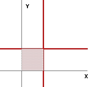
For example the feasible region for the following constraints

Linear Programming Problems

Simplex Method

• Each variable should be contrained to be non-negative; and
• All other constraints should be linear expressions less than or equal to some positive constant; and
• We choose to maximize rather than to minimize the objective function

If the feasible region is bounded, then all we need to do to satisfy the first condition is to shift our variable to put the feasible region into the first octant. If the second condition is not met, we can reorganize the constraint that causes the problem to put all the variables on the left and the constant on the right. If the constant is negative, multiply both sides by -1. If the third condition is not met, we just use the negative of the original objective function as the new objective function.

Slack Variables

If we have a constraint of the form

can be converted to a linear equation in one extra variable, s (a "slack variable") subject to one additional non-negativity constraint on s

where s measures the slack we have in getting from the original inequality to equality.

Tableaux

Under the constraints

Maximize

The same variable names appears again and again. We can organize all the information into a table, which we call a "Tableau", with a column heading for each variable x₁, x₂, x₃, ..., s₁, s₂, s₃, ..., s₃, P, and another two columns, one for each right hand side and one to keep track of a a variable from each row called a "basic variable", which starts as the slack variable for each. We take the objective function and subtract P from both sides and get

Running the Simplex Method on a Tableau

The Simplex Method uses a tableau as a way to explore the values of the objective function at one corner of the feasible region at a time walking to higher and higher values until it reaches the highest value. The steps are as follows:

1. Set up the tableau with the slack variables as the initial basic variables
2. If there are no positive elements in columns for varibales or slack variables in the bottom row (the objective function) STOP, you are done.
3. If there are any positive elements in the bottom row in columns for variables or slack variables , make one of the columns that contains a positive value in the bottom column, the PIVOT COLUMN (it is usually a good idea to take the column with the largest value in the bottom row).
4. For each row (but not the row of the objective function) with a positive entry in the PIVOT COLUMN, divide the value of the RHS by that positive entry. Don't change the RHS, just keep track of the quotient for each row with a positive entry in the PIVOT COLUMN. Make the row with the smallest quotient the PIVOT ROW.
5. Call the element in the PIVOT ROW and PIVOT COLUMN, the PIVOT ELEMENT
6. Divide every element in the PIVOT ROW, including the RHS, by the PIVOT ELEMENT so that the new PIVOT ELEMENT is now 1.
7. For every other row, including the row of the objective function) subtract whatever multiple of the new PIVOT ROW is needed to force a zero into the PIVOT COLUMN for that row.
8. Change the basic variable for the PIVOT ROW to be the variable of the PIVOT COLUMN.
9. go back to step 2.

When you are done, if you have negative right hand sides for anything other than the objective function row, there is no feasible solution, but if you have non-negative right hand sides, just read off the RHS column as the values for the BV column variables and read off the negative of the RHS for the last row as the maximum value of the objective function.

What the Results of Simplex Mean

When there are no further positive elements in the bottom row, the RHS column gives the values for the basic variables for a solution, including a value for the objective function. For each of the non-basic variables, the value at the solution is zero. The negatives of the (negative) values in the last row for those variables is called the "reduced cost", and shows how much the payoff would be reduced by a unit increase of that variable. If the variable involved is a slack variable, the reduced cost is called the "shadow price". If a slack variable is assigned a zero value in the solution the corresponding constraint is called "tight" or "binding", because the limit of the constraint was hit, and having more of the resources involved in that constraint might allow for a larger payoff.

If the righthand side of a constraint can be increased by a certain amount without changing the reduced costs (the shadow prices) of any of the slack variables, that is called an "allowable increase". Similarly, if the righthand side of a constraint can be decreased by a certain amount without changing the reduced costs (the shadow prices) of any of the slack variables, that is called an "allowable decrease".

The allowable increase for a non-basic variable is the reduced cost.

If a slack variable has a non-zero value, the corresponding contraint is called "non-binding", and there is nothing to be gained by trying to relax that constraint.